22 Nov 2015

Bootstrapping made simple

Resampling is an absolutely crucial technique when fitting models to data. I've read (and appreciate) arguments that a train/test split of data may not be the most sensible thing to do, as you lose data which could be used to build your model. Also, the key point of this argument is that if your resampling is done well, your model evaluation based on resampling should deliver the same answer as your test set (provided the training set is representative of the test set).

There are several usual techniques, such as k-fold cross validation, leave-one-out cross validation, and bootstrapping. I'm going to focus on the bootstrap for this post, but that doesn't neccesarily mean it's always the most appropriate technique to use. All have a play-off between bias and variance that needs to be considered, and for large samples of data, some techniques can be significantly more computationally demanding (you need to be seriously patient to attempt using leave-one-out cross validation for a large data set, for example).

The R caret package makes cross validation trivial to include in your modeling, thanks to the easy syntax of caret::train() and caret::trainControl(). I would always use caret for a 'real' model over what I am about to present.

Overview

Now firstly, a little disclaimer. I do not claim to be an expert on bootstrapping by any stretch of the imagination- I have touched upon it in a few statistics courses, and I am fully aware there is a rich and deep statistical theory behind the technique. That being said, although my understanding is simple and intuitive, it is certainly sufficient for applictions where I need resampling or to generate distributions.

So anyway, how does bootstrapping work in the context of resampling? It's actually fairly straightforward. Bootstrapping amounts to sampling with replacement. What you do is sample rows from your data, where some rows will be selected more than once, and others not at all. This gives you what is known as an in-bag and out-of-bag sample. A neat thing about bootstrapping is that you can immediately test a model built on the in-bag samples upon the out-of-bag samples.

What you typically do is repeat this process, and evaluate a peformance metric (such as RMSE) using the model built using the in-bag samples on the out-of-bag samples. This way, you build up a distribution of your metric, and can easily compare peformance between two models. Its that simple!

Implementation

A simple bootstrapping function can be written in R making use of subsetting. Here is my implementation (you can get the entire R script here):

#
# basic bootstrap function. Formal arguments are
# an input dataframe and the number of bootstrap 
# resamples desired
#
bstrap <- function(df, samples = nrow(df)) {
  #
  # sample row indices with replacement
  #
  inBagRows <- sample(nrow(df), nrow(df), replace = TRUE)
  #
  # define the in bag and out of bag rows
  #
  inBag <- df[inBagRows, ]
  OOB <- df[-inBagRows, ]
  #
  # output
  #
  return(list(inSample = inBag,
              outSample = OOB))
}

I could probably have made it more lightweight by just outputting the in-bag and out-of-bag row indices for subsetting, rather than copies of the data frame. However, for illustration purposes I think it is a little more clear this way.

An example

For the sake of a concrete example, lets fit two models to some simulated data. The data is defined below: it is quadratic, with random noise with standard deviation 10 added to each term.

#
# simulate some data - quadratic with normal noise 
#
x <- seq(1, 10, 0.1)
y <- 2 * x ^ 2 + x + rnorm(x, 0, 10)
#
# build up a data frame of predictors and outcome
# include linear and quadratic terms in x
#
sim_data <- data.frame(x1 = x,
                       x2 = x ^ 2,
                       y = y)

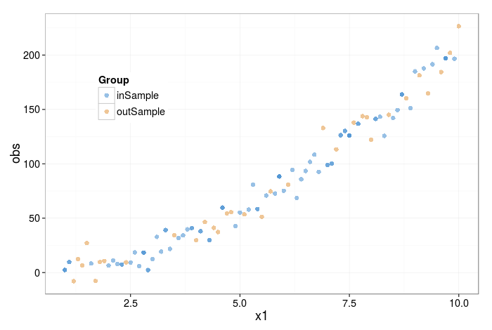
The figure below shows a bootstrap sample of the data; orange points are 'out-of-bag' (i.e. not selected at all), and blue points are in-bag. Note that in-bag points may have been selected more than once. There is, in fact, a 63.2% chance of each point being represented at least once.

How do we proceed from here? A single bootstrap resample would now take the in-bag data, fit a model to it, and evaluate the model on the out-of-bag samples (e.g. calculate the RMSE error for the predictions on the out-of-bag samples). The idea is to repeat this many times, so that a distribution can be built up. You can then analyse this distribution of the peformance metric to make informed decisions about which model to select.

The code below peforms multiple resamples, and stores the RMSE from two hypothesised models; one which is just linear in x, and one that contains a quadratic term.

#
# data frame to hold resamples
#
resamples <- data.frame(rmse = rep(NA, 500),
                        model = rep(c(lin, quad), 250))
#
# This loop performs 250 bootstrap resamples, fitting
# two different hypothesised models for the data.
#
for (i in seq(1, 500, 2)) {
  tmp <- bstrap(sim_data)
  # fit a linear model
  fit <- lm(obs ~ x1, data = tmp[[1]])
  fit2 <- lm(obs ~ x1 + x2, data = tmp[[1]])
  OOB <- tmp[[2]]
  #
  # extract predictions with predict.lm() to compare
  # to the correct result
  #
  linPred <- predict(fit, OOB[, 1, drop = FALSE])
  quadPred <- predict(fit2, OOB[, 1:2, drop = FALSE])
  correct <- OOB[, 3, drop = TRUE]
  #
  # rmse of out-of-bag samples
  #
  resamples[i, 1] <- sqrt(mean((linPred - correct) ^ 2))
  resamples[i + 1, 1] <- sqrt(mean((quadPred - correct) ^ 2))
}

We can plot the distribution of the results with a histogram or box plot (I present the latter here).

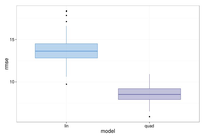
A visual inspection shows the quadratic model has a distribution with a rmse centered significantly below the model which only includes a linear term.

Statistical testing on the resamples

The last question is, how should we formally resolve which model is better? My approach is to use a hypothesis testing. We can use the following syntax to run the t-test:

#
# Peform a t-test with this syntax. A paired test
# is used, as for every resample both models are fitted.
#
t.test(resamples[resamples$model == lin, 1],
       resamples[resamples$model == quad, 1],
       paired = TRUE,
       alternative = two.sided)

The rule of thumb is that if you cannot reject the null, choose the most parsimonious model- which will likely be easier to implement and be far more interpretable. However, in this case (as expected, as we know the functional form) the model including the quadratic term far outperforms the model including only the linear term: the p-value is virtually zero.

Other Thoughts

So there we have it; a simple demonstration of applying bootstrapping as a resampling tool for fitting models. One warning about the bootstrap is that it can result in biased results. There exist modifications, such as the 632 method, which serve to eliminate this bias, but that is another discussion for another time.

I'll reiterate one point I made earlier: I suggest you turn to caret and use it's built in resampling options if you want to apply bootstrap resampling for real modeling using R. None the less, I hope this was an enlightening read if you have never applied the bootstrap in the context of machine learning, or never thought about how it works!

TL;DR- a simple demonstration of using the bootstrap for resampling when fitting models. Check out the code here.