12 Jul 2016

Class imbalance in classification models

Severe class imbalance can be an absolute pain. Take the example where a population only has 1% being of the class of interest. We can obtain an accuracy of 99% by predicting all samples to be of the majority class- which is utterly useless if the minority class is of interest. Training models where the outcome is disproportionate can be tricky. Taking our example, if we train models using accuracy as the evaluation metric, our model will likely have a very high specificity, but an abysmally bad sensitivity.

So here we go: some useful tips for dealing with situations like this! I used the adult dataset (its in the arules package, or you can get from the UCI machine learning repository) to investigate this, but the techniques I will discuss are pretty general, and can be applied to any data set. I used C5.0 as my candidate model throughout, but there is nothing stopping you using others as you investigate your problem.

The dataset is balanced with approximately 75% having an income classed as small, and 25% classed as large. Lets say, for sake of argument, that we are using this data to identify customers with high salaries so that we can target them for a marketing campaign. To focus our campaign effectively, we need to be able to identify these customers.

As a final point before getting started, I will direct you to Kuhn and Johnson's Applied Predictive Modeling if you want a much more in-depth discussion on the subject of class imbalance.

Setup and Baseline

As the emphasis of this post is class imbalance, I wont dwell upon data exploration or pre-processing. Check out the script in the repo that will process the data set into the one I used for modelling.

Im going to tune models using the trusty caret::train function. First, lets define a control object, summary functions, and the training grid for for training the C50 model:

# 
# define summary function (wrapper around caret helper functions)
fiveStats <- function(...){
  c(twoClassSummary(...), defaultSummary(...))
}
# 
# set up control for caret:: train
ctrl <- trainControl(method = cv,
                     number = 3,
                     classProbs = TRUE,
                     savePredictions = TRUE,
                     summaryFunction = fiveStats)
#
# define the training grid for the C50 model
c50Grid <- expand.grid(trials = c(1:9, (1:10)*10),
                       model = c(tree, rules),
                       winnow = c(TRUE, FALSE))

And now to train, defining ROC as the evaluation metric for determining tuning parameters:

# 
# set seed and train model
set.seed(476)
c50TuneBaseline <- train(x = inputTrain,
                         y = outcomeTrain,
                         method = C5.0,
                         tuneGrid = c50Grid,
                         verbose = FALSE,
                         metric = ROC,
                         trControl = ctrl)

This baseline model has a senstivity of 0.6722 and a specificity of 0.9312 on the test set. In other words, our model is much better at identifying small incomes than large (which might be expected due to the class imbalance).

Train on a metric that emphasises the class of interest

As we saw from the baseline model, the sensitivity is very poor: we struggle to identify the customers of interest in the minority class. A simple first step to improve our ability to identify these customers is to train our model to optimise the metric of interest. This can be achieved simply with the syntax:

# 
# set seed and train model
set.seed(476)
c50TunSens<- train(x = inputTrain,
                   y = outcomeTrain,
                   method = C5.0,
                   tuneGrid = c50Grid,
                   verbose = FALSE,
                   metric = Sens,
                   trControl = ctrl)

On the test set, a sensitivity of 0.6509 was obtained, with a specificity of 0.9347. In this case, the model sensitivity is actually worse than the baseline model, which emphasises the severity of the problem we are facing.

Alternative cutoffs

One nice, easy to implement trick to combat the effects of class imbalance is to change the probability cutoffs used to define the class. We can choose to be optimistic or pessimistic. For example, an optimist might consider the prediction to be the class of interest if the probability is over 30%, rather than the usual cutoff of 50%.

The pROC package comes with the functionality to determine suitable cutoffs. If you think about a perfect ROC curve, it represents a model with sensitivity and specificity of one. A reasonable approch is to select the cutoff that is the point on the ROC curve geometrically closest to the perfect model (i.e. top left point of the plot).

This is a situation where the validation set is required: we should determine our cutoff on the validation set, and apply this to the test set. This can be achieved with the syntax:

# 
# create object ValPredProb by predicting validation set
# postive class (gt50) probabilities using C50TrainSens
C50ROC <- pROC::roc(outcomeVal,
                    ValPredProb,
                    levels = rev(levels(outcomeVal)))
#
# determine the new cutoff to be used on the test set
C50Thresh <- pROC::coords(C50ROC, x = best, best.method = closest.topleft)
newPredictions <- factor(ifelse(testPred > C50Thresh[1],
                                gt50, le50))

On the test set, a sensitivity 0.8469 and a specificity of 0.8265 was obtained. Compared to the baseline model, some specificity has been sacraficed to achieve a much greater sensitivity.

Up and Down Samping

When class imbalance has been identified, one relatively simple method to remedy it is by up or down sampling. In its most straightforward form, downsampling is equivilant to randomly removing points in the majority class until the classes are balanced. Up sampling is equivalent to duplicating randomly selected points in the minority class until the class distribution is balanced. The model is then trained on this data where the classes are balanced.

The caret library contains functions to do just this, which can be achieved with the syntax:

#
# set seed and up sample with the following syntax:
set.seed(123)
upSampledTrain <- caret::upSample(x = inputTrain[, fullSet],
                           y = outcomeTrain,
                           yname = earning)
#
# ensure the classes are now balanced
prop.table(table(upSampledTrain$earning))

The syntax for down sampling with caret::downSample() is identical. As a word of warning, when down sampling I would check for zero variance predictors: if you have near-zero variance predictors in your input, you stand a risk of exhasperating the issue when down sampling.

When up sampling, a sensitivity and specificity of 0.7483 and 0.8847 were obtained, and when down sampling a sensitivity and specificty of 0.8661 and 0.7979 were obtained.

Cost-sensitive models

The final method I will discuss is usage of models that can implement different weights on false positive or false negative predictions when training. This modifies the cost function that is being used when fitting the model. Think of it as fitting your model imposing that a false positive is X times worse than a false negative, or vice versa.

Not all models have this functionality implemented (although I imagine it is a reasonably straighforward modification to implement in any learning algorithm). C50 does, however, so can be used as an example. One quick point is that C50 cannot generate class probabilities when using unequal case weights. Therefore, we should update our control function:

#
# define a new summary function that does not calculate ROC curves 
# and corresponding AUC (as probabilities are required for this)
fourStats <- function (data, lev = levels(data$obs), model = NULL) {
  accKapp <- postResample(data[, pred], data[, obs])
  out <- c(accKapp,
           sensitivity(data[, pred], data[, obs], lev[1]),
           specificity(data[, pred], data[, obs], lev[2]))
  names(out)[3:4] <- c(Sens, Spec)
  out
}
#
# copy the old control object, and update the summary function
ctrlNoProb <- ctrl
ctrlNoProb$summaryFunction <- fourStats
ctrlNoProb$classProbs <- FALSE

Now we can define the weights in a matrix. Here, I define a false negative to be 10 times 'worse' than a false positive.

#
# weights for model tuning
c5Matrix <- matrix(c(0, 10, 1, 0), ncol = 2)
rownames(c5Matrix) <- levels(outcomeTrain)
colnames(c5Matrix) <- levels(outcomeTrain)
#
# can no longer optimise based on ROC AUC
# choose kappa statistic
C5Cost <- train(x = inputTrain[, fullSet],
                y = outcomeTrain,
                method = C5.0,
                metric = Kappa,
                cost = c5Matrix,
                tuneGrid = c50Grid,
                verbose = FALSE,
                trControl = ctrlNoProb)

On the test set, a sensitivity of 0.8372 and a specificity of 0.8296 were obtained.

Summary

We can do a quick plot to compare the resulting sensitivities and specificities of each model.

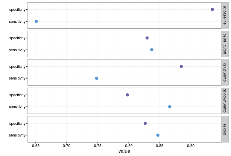
What we observe is a tradeoff between sensitivity and specificity. As to which technique should be preferred: the modeller should make that decision based on the needs of the situation. Clearly using the weighted model and alternate cutoffs produce the most 'balanced' model sensitivity and specificty, but it may be of more interest to choose the down sampled model that gives the best sensitivity. Depending on the situation, different techniques might be preferred.

So there we have it: several methods to tackle situations where moderate to severe class imbalance is encountered. Thanks to the caret package, these remedies are easy to implement, and can vastly improve the performance of predictive models.

TL;DR- I investigated several ways to remedy class imbalance in a binary classification problem. My scripts are here.