
20 May 2016
Model Ensembles: Regression
Since my post on various flavours of stacking I have been doing a fair bit of thinking about model ensembles. The idea of combining predictions together to enhance performance is nothing new- techniques such as bagging and boosting have been around for a while. I've decided to get serious with the notions of stacking and blending, two interesting ways to combine predictions, perhaps from very different classes of model, into an ensemble to create predictions better than any individual model in the ensemble.
My reading on the subject consisted of several papers in academic journals. As per my previous post, this paper by Breiman is a good reference for stacking (although I have found that stacking using the elastic net tends to perform better than combining models whilst enforcing non-negative weights). These papers by Caruana et al are a really interesting read on blending, albeit in the context of classification. Finally, this article by Dietterich gives a really intuitive description of why ensemble models tend to perform well.
For once, I'm not making my implementation publicly available... yet. I want to test and refine my approach, and try out on a few more datasets. I may even consider releasing it on CRAN if I feel it gets to the stage where it can be useful for other people!
Types of regression ensemble
I'm going to be considering two types of regression ensemble. Firstly, stacking. The basic idea is to generate predictions on a validation set from each model in the ensemble, and use a method to combine these 'level one' predictions together. I'm going to use the elastic net, as it will be able to combat the fact that the level one predictions are inherantly correlated with one another (they are predicting the same thing), but yet is still a relatively simple linear regression technique. The learned coefficients from the validation set can then be used to combine the predictions of all the models in the ensemble on the test data.
Secondly, I will be considering blending. This is actually a relatively simple idea. In it's most basic form, its essentially model averaging (i.e. for N models making predictions on m test samples, simply average the N predictions for each sample). Caruana advocates a robust method for building the blended ensemble with a hillclimb approach, iteratively adding models to the ensemble, choosing at each iteration the model that reduces the error on the training set the most. He also advocates some neat tricks in the finer details, such as selecting models with replacement and bagging. I suggest that you have a read of the paper, as my approach is losely based on this implemenation (you will see later that I have an additional backwards selection step to remove models that don't improve the performance of the ensemble).
Defining an S4 class
I'm getting in the habit of defining S4 classes in my R packages for tasks like this. What do we actually need for our ensemble?
Now, I like to use caret to build my models. It nicely takes care of model training, resampling, and is full of useful helper functions. What do we need to keep then, for our objects of class 'ensemble'? I've whittled it down to a few things.
- a list holding the predictions of each model on the validation set, plus the actual validation outcome and some performance metrics for each model
- a list holding some perfomance metrics of the ensemble on the validation set
- a string to denote whether the ensemble is for regression or classification
- a string to denote the ensemble type (stack or blend)
- a list that holds the details of the ensemble method, and crucially, the ingrediants neccessary for making predictions
#
#' S4 class definition for a model ensemble
#'
#' @slot type character string. can be
regression
or
#' classification
.
#' @slot valPerf list holding predictions and performance
#' of each model on the validation set.
#' @slot valPerfEnsemb the performance of the ensemble on the
#' validation set
#' @slot ensembleType type of ensemble. Can take values
#' stack
, blend
#' @slot ensembleMethod list holding information describing
#' how the ensemble is created.
#'
setClass(
Class = ensemble
,
slots = list(
type = character
,
valPerf = list
,
valPerfEnsemb = list
,
ensembleType = character
,
ensembleMethod = list
)
)
I will also want some handy generics for this class: a summary, show, plot, and predict generic is crucial to define. For example, the plot generic should represent the influence of each model in the ensemble. I will discuss these shortly!
Building Ensembles
The constructor for the ensemble class is so key to the entire process. It's easy to describe how it works. The code is the following:
#
#
ensembleBuild <- function(models, type =
regression
,
inputVal, outcomeVal,
ensembleType = stack
, options = NULL) {
#
# make predictions on validation set
valPred <- vapply(
models,
function(x) {
inputSet <- names(x$trainingData[1:(ncol(x$trainingData) - 1)])
predict(x, newdata = inputVal[, inputSet])
},
numeric(nrow(inputVal))
)
colnames(valPred) <- paste('model_',
sprintf(%03d
, 1:length(models)),
sep = )
#
# perfomance metrics on validation set
valPerfMetric <- data.frame(
model_id = paste('model_', 1:length(models), sep = ),
method = vapply(models, function(x) x$method, character(1)),
RMSE = apply(valPred, 2, caret::RMSE, outcomeVal),
R2 = apply(valPred, 2, caret::R2, outcomeVal)
)
#
# stacked regression
# use the elastic net to combat correlated predictors
# options are training parameters to elastic net model
if (ensembleType == stack
) {
ensembleMethod <- buildStack(
valPred,
outcomeVal,
options = options
)
}
#
# blended model
# options control bagging process
if (ensembleType == blend
) {
ensembleMethod <- buildBlend(
valPred,
outcomeVal,
numModels = length(models),
options = options
)
}
#
# build object of class ensemble and return it
return(new(
Class = ensemble
,
type = type,
valPerf = list(predictions = valPred,
actual = outcomeVal,
performance = valPerfMetric),
valPerfEnsemb = list(RMSE = ensembleMethod$valRMSE,
R2 = ensembleMethod$valR2),
ensembleType = ensembleType,
ensembleMethod = ensembleMethod)
)
}
#
#
First, we make predictions on the validation set using the objects of class train. Using the true validation outcome, we can calculate the perfomance metrics on the validation set. Next, we call the appropriate function, depending on whether we want a stacked or blended ensemble. Finally, we return an object of class ensemble, filling in the slots appropriately.
Stacked models are easy to build. The buildStack() function is essentially a wrapper around caret::train(), training an elastic net model with the model predictions on the validation set as the input, and the true validation outcome as the target. The options argument passes arguments to this function, should the user want to define them.
Blended models are conceptually easy to build, but can be a bit tedious to code up. My implementation is based loosely on Caruana's, but I add an optional (greedy) backstep phase after every bagging iteration. This works backwards through the models that have been added to the ensemble from that bagging iteration, and removes those that result in the RMSE of the ensemble on the validation set to decrease.
Test 1: Physicochemical Properties of Protein Tertiary Structure dataset
I wanted a data set with a fairly large number of entries, so that I could hold out a large test set to get a good idea of the ensemble performance. I stumbled accross the Physicochemical Properties of Protein Tertiary Structure data set on the UCI machine learning repository. The aim is to regress upon the surface area using various meaurements as predictive inputs.
The data set consist of 45730 observations of 10 variables (9 predictors and the outcome). Perfect. A little investigation reveals that some rows are full duplicates, and some have duplicated inputs, but different outcomes. These need addressing, as if there are duplicates in the train, validation and test set, this may result in an over optimisitic measure of model performance. My strategy is to remove (all but one) of each of the full duplicates, and for those with duplicated inputs but different outcomes, take the average response. Note that I only do this for the train and validation set- the test set is ALWAYS left as is! I like to think that it's like a Kaggle competition- imagine you have no access at all to the test set, other than being able to assess the performance of your predictions.
I use the following syntax for my data splitting and processing of the train and validation data:
#
# partition data
#################################################
library(caret)
library(dplyr)
#
set.seed(1234)
inTrain <- createDataPartition(CASP$RMSD, p = 0.7, list = FALSE)
trainDat <- CASP[inTrain, ]
#
# remove full duplicates: lose 865
trainDat <- trainDat[!duplicated(trainDat), ]
#
# average the outcome for duplicate features (i.e. input same, outcome different)
trainDat <- trainDat %>%
  group_by(F1, F2, F3, F4, F5, F6, F7, F8, F9) %>%
  summarise(RMSD = mean(RMSD))
#
# lose 28. convert back to class data frame
trainDat <- as.data.frame(trainDat)
#
# Split up the input/ outcome
inputTrain <- trainDat[, 1:9]
inputTest <- CASP[-inTrain, 2:10]
outcomeTrain <- trainDat[, 10]
outcomeTest <- CASP[-inTrain, 1]
#
# Split the train into train/ validation
set.seed(1234)
inVal <- createDataPartition(outcomeTrain, p = 0.2, list = FALSE)
inputVal <- inputTrain[inVal, ]
inputTrain <- inputTrain[-inVal, ]
outcomeVal <- outcomeTrain[inVal]
outcomeTrain <- outcomeTrain[-inVal]
This results in 24894 observations in the training set, 6225 in the validation set, and 13718 in the test set.
I must confess, I am a little confused by some of the measurements- for example some surface areas are exactly zero. Physically, what does this correspond to? But anyway, I will just happily ignore this quirk (the documentation is poor/non-existant), and continue!
Right, this data set is pretty easy to preprocess- we have no categorical data. The first step is to do some visualisations. Let's start with the relationship between the inputs and the outcome:
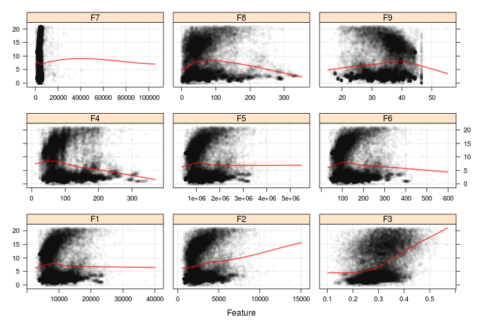
Oh gosh, certainly doesn't look like there are clean, general trends in that data set! Looking at the outcome in isolation (not shown here) the distribution is bimodal, which suggests that nonlinear or nonparametric models may perform better than linear models The most prominent is in feature F3. Something tells me we are going to struggle to get tiny RMSE when fitting models...
Looking at between-predictor correlations, we see that there is a high (almost full) correlation between F1 and F5. We will remove one of these, even for models that can perform internal feature selection. I define a full and reduced set of predictive inputs, one for models that are resilient to correlated or non-informative predictors, and one for models that are not. The syntax to do this is easy, thanks to caret::findCorrelation:
#
# investigate correlation- set a threshold of 0.9 for
# reduced set, 0.99 for full set
trainCorr <- cor(inputTrain)
highCorr <- findCorrelation(trainCorr, cutoff = 0.9)
fullCorr <- findCorrelation(trainCorr, cutoff = 0.99)
highCorrNames <- names(inputTrain)[highCorr]
fullCorrNames <- names(inputTrain)[fullCorr]
#
# full and reduced set of predictive inputs
fullSet <- names(inputTrain)[!names(inputTrain) %in% fullCorrNames]
reducedSet <- names(inputTrain)[!names(inputTrain) %in% highCorrNames]
#
Training can then begin! For a selection of models, I start by using caret::train() with appropriate CV (5-fold CV in this case) to find optimum values for the model tuning parameters. With this information in mind, I can train models using different choices of training parameter (not neccessarily the optimum) to build up a collection of models for the ensemble. As an explicit example, I train here 3 random forest models using mtry = 4, 5 and 6 for ntrees = 2000:
#
# assume rfGrid and rfCtrl defined
set.seed(1234)
rfTrain <- train(x = inputTrain[, fullSet],
y = outcomeTrain,
method =
rf
,
tuneGrid = rfGrid,
ntrees = 2000,
trControl = rfCtrl)
plot(rfTrain)
#
# best tuning param (mtry) are 4, 5, and 6
# build a list of three models corresponding to these values
#
rfCtrl <- trainControl(method = none
)
rf_models <- lapply(seq(4, 6), function(x) {
train(x = inputTrain[, fullSet],
y = outcomeTrain,
method = rf
,
ntrees = 2000,
tuneGrid = data.frame(mtry = x),
trControl = rfCtrl)
})
#
The models I consider are:
- K nearest neighbors
- MARS
- cubist
- random forest
- stochastic gradient boosted trees
- extereme gradient boosted trees
- support vector machine (radial basis kernal)
- support vector machine (polynomial basis kernal)
- (averaged) neural networks
And away I go: I firstly make a list of these models, and then combine them into an ensemble using the ensemble constructor. But wait, there are some problems!
Feedback and Improvements
User feedback is incredibly useful- even if you are the user! I had numerous minor issues that I tweaked, but there were some more significant design choices that needed to be considered. I had some concerns after building my initial ensemble:
- storing all the models of class train can use up a huge about of memory- the random forest models, for instance, are hundreds of megabytes in size. This will cause you to quickly run out of RAM.
- what happens if objects of class train are unavailable? For instance, what happens if you are collaborating with a friend who prefers using Python to R? Or perhaps another friend who transforms the data set before fitting models? Restricting the user to building objects of class train seems to be too prohibitive.
What is a good solution to this? I didn't want to remove the option to feed in a list of models of class train, so I defined a second constructor. The ensembleBuildSlim() constructor simply requires a data frame of the predictions on the validation set, rather than the list of models. This significantly reduces the memory needed. Further, a friend could email you their model predictions in a simple flat text file, and you could read it in to R and append their predictions on the validation set to your own.
Well, I found this to be a lot more satisfactory. As an example of 'non-compatible' objects of class train, I transformed predictors by adding 1e-6 to each value (so that I can transform zero's), and then a Box-Cox transformation to the predictive inputs in the preprocessing stage. I would have require two sets of validation inputs, the original and the offset version, if I was to make my predictions on the validation set in the constructor function. Much easier just to make the predictions, and pass these in!
Test 2: Physicochemical Properties of Protein Tertiary Structure dataset revisited
Right, so time to build an ensemble, now that the tweaks are performed! I built up a total of 68 models different classes, of varying performance. The 'best' single model was a cubist model, which had a RMSE of 3.608713 and an R2 of 0.6543543 on the validation set. I build a stacked and blended model with the syntax:
# valPredComb is a data frame where each column corresponds
# to model predictions on validation set
#
# In the blending process, I perform 1000 bagging iterations,
# where at each iteration I initialise the selected models
# with the three best models in the bag, and select a maximum
# of 15. I perform a backstep phase, removing models that
# do not improve the full ensemble
model_blend <- ensembleBuildSlim(type =
regression
,
valPred = valPredComb,
outcomeVal = outcomeVal,
ensembleType = blend
,
options = list(NBag = 1000,
NInit = 3,
NSelect = 15,
backStep = TRUE,
seed = 123))
#
#
# The stacked model uses the elastic net to combine the models
model_stack <- ensembleBuildSlim(type = regression
,
valPred = valPredComb,
outcomeVal = outcomeVal,
ensembleType = stack
)
#
Well great, there we go! Two objects of class 'ensemble'. Time for a quick tour of the generics!
The summary generic gives us some general information, including the RMSE and R2 of the ensemble on the validation set. The blended model scores a RMSE of 3.518956 and an R2 of 0.6696131, and the stacked model an RMSE of 3.501856 and an R2 of 0.6723064. So far, so good. The summary also tells us how many models were included in the ensemble- for the stack, it counts the number of non-zero coefficients from the elastic net, and for the blend, it counts the number of unique models in the mix.
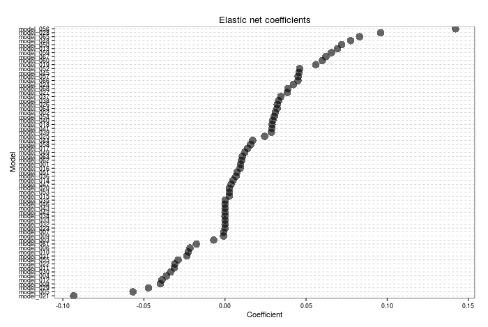
The plot generic will display either the fitted elastic net coefficients corresponding to each model, or the relative proportion of the blend corresponding to each model. The blend proportion must add up to 1, and note that I do not enforce non-negativity in the model coefficients, like Breiman advocates in his paper. Here is an example of the plot generic for the stacked model- note that some coefficients are exactly 0 (i.e. not included in the ensemble). I need to give some thought as to what a negative coefficient actually corresponds to in this context...
The predict generic is perhaps the most important! The user must input the predictions of the individual models on the test set, and the generic will combine them to produce the ensemble prediction:
# syntax for the predict generic.
# The user must provide a data frame of the model
# predictions on the test set, IN THE SAME ORDER
# as they were provided when building the ensemble
predict(model_stack, testPredComb)
#
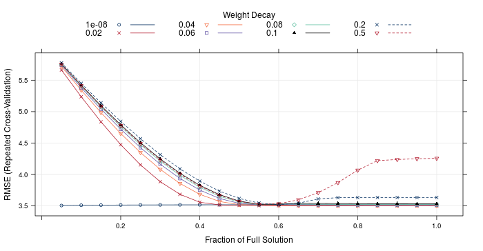
I've also included a couple of custom generics: an accessor valPerf() that returns the perfomance of the individual models on the validation set, as well as the ensemble coefficients/ proportions, valPlot() that allows a visualisation of the predictions vs true value for the validation set for each model, and ensembPlot() that will either plot the elastic net resamples for a stacked ensemble, or the validation RMSE as a function of number of models for the blended ensemble. As an example, ensembPlot(model_stack) will yield:
Right, enough showing off all the generics. How well do ensembles actually do? Lets look at the RMSE and R2 on the test set. The test set consisted of 13718 observations, so should provide a good indicator of true model performance.
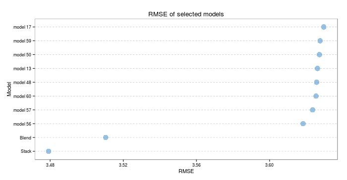
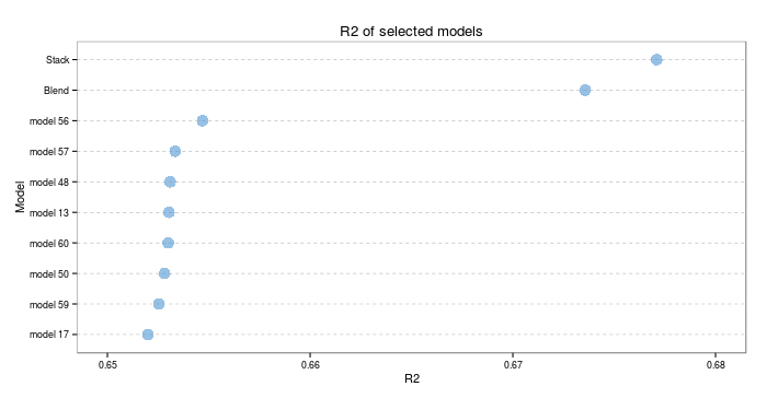
I hope those visualisations, in themselves, are proof that this was worth the effort. Both types of ensemble significantly outperform the next best individual model (which was a cubist model). On the test set, the stacked model scores an RMSE of 3.479163 and an R2 of 0.677094. The blended model scores an RMSE of 3.510419 and an R2 of 0.6735671. The best individual model scores an RMSE of 3.618323 and an R2 of 0.6546914- we have outperformed that threshold significantly!
Next steps
Whew, now that was the culmination of a fair few evenings effort! I'm pretty pleased with the results. I'm keen to play around a bit more- perhaps I will set a target to obtain an R2 of 0.7, and see if I can achieve that. That's if I'm not approaching the irreducible model error...
I think my next step is to thoroughly document the package, add some tests, and get to a stage where I am happy to release it on my github (it's currently hidden away in a private repo on Bitbucket), and eventually (if I feel brave) CRAN.
And then, the next real step is to extend the capabilities to classification models! I think I will tackle that once I have the regression side of things working nicely.
TL;DR- I've started developing an R package to create model ensembles. The results are promising so far!