Ensemble Models: Various Flavours of Stacking

16 Mar 2015

I recently stumbled across an article on the subject of Feature-Weighted Linear Stacking (FWLS) that was a by-product of the well known million-dollar Netflix Prize. I was well aware of the notion of 'stacking' or 'blending' predictions to produce higher quality predictions, having been introduced to the concept by Jeff Leek's Machine Learning Course, but it is only now that I have gotton around to investigate the idea myself.

A bit more digging yeilded the classic paper on the subject by late, great, Leo Breiman. I'll be focusing this blog mainly on my interpretation of the ideas presented in his paper, and touch upon FWLS breifly as well.

I will be focusing my investigation around a fairly straightforward regression problem (apologies to anyone who was expecting a collaborative filtering example, in the spirit of the Netflix Prize). Max Kuhn and Kjell Johnson's Applied Predictive Modelling Book dedicates a chapter around a case study optimising the compressive strength of concrete mixtures (a fascinating read, highly recommended), and as the data set is fairly 'nice', I will borrow it for this example! It can be loaded with

#
# load the library and the data
#
library(AppliedPredictiveModeling)
data(concrete)

So let's dive in! As always, my scripts are available on my github, should you like to snoop, criticise, or copy my approach!

Explore data set

The concrete data set was the focus of a research paper by Yeh, who demonstrated how 'mixture design' experiments can be led from predictive modelling. Essentially, he aimed to build a model to predict the compressive strength of concrete based upon the mix, and then optimise the mix to suggest what may produce the strongest concrete. The chapter dedicated to the problem in Applied Predictive Modeling is fascinating, and I suggest you read it!

The first step is explore the data. Following the advice in the book, I perform an initial check for missing data or duplicates. In this case we find no missing data, but there are some duplicate rows. I chose to seperate these into two types: those with duplicate inputs (mix ingredients) and outcome (compressive strength), and those which have duplicate inputs but different outcomes. I though these two types of duplicates were useful to distinguish. Those 'full' duplicates can be removed- they give us no useful information, and may introduce bias in the model.

Those with identical mixes, but different outcomes are interesting, and perhaps useful from another perspective. If identical ingredients produce different results, does this tell us something about the irreducible error in our model? That is, there is some randomness and uncertainty in the results. If you measure anything multiple times, you should find your measurements sit in a (probably gaussian) distribution around the mean expected value (the variance will be small if you make very good measurements). In this case, slight uncertainties in the mix as well can exhasperate the problem. Therefore, the outcome isn't perfect. This is one example of why overfitting is dangerous- if you fit your model to the noise and uncertainty in the outcome, it won't generalise well!

Anyway, I thought it would be interesting to see what the mean standard error was for those mixes with duplicate inputs but different outcomes. I got a value of 3.89 using the following syntax:

#
# remove full duplicates
#
concrete <- concrete[!duplicated(concrete[, 1:9]), ]
#
# which just have duplicated input (not outcome?)
#
concrete[duplicated(concrete[, 1:8]), ]
#
# here is an experiment for what is irreducible error
# using dplyr
#
concreteIrreducible <- concrete %>%
  group_by(Cement,
           BlastFurnaceSlag,
           FlyAsh,
           Water,
           Superplasticizer,
           CoarseAggregate,
           FineAggregate,
           Age) %>%
  summarise(stderr = sd(CompressiveStrength) / sqrt(n()))
#
#
mean(concreteIrreducible$stderr, na.rm = TRUE)

This probably gives us hints around the best performance we can expect; if repeat measurements vary this much, we wouldn't, for example, expect a RMSE on a test set significantly lower than this.

I resolved the duplication issue by taking the average outcome for those duplicated mixtures. Next, I perform a train-test split (70% in the training set- 696 samples), and then further split my test set into a test and validation set (146 samples in each). We can easy visualise the training data using caret::featurePlot() with the syntax:

#
# I steal Max Kuhn's settings as he is waaay better 
# at using lattice graphics than I am
#
theme1 <- trellis.par.get()
theme1$plot.symbol$col = rgb(.2, .2, .2, .4)
theme1$plot.symbol$pch = 16
theme1$plot.line$col = rgb(1, 0, 0, .7)
theme1$plot.line$lwd <- 2
trellis.par.set(theme1)
#
# caret::featurePlot makes plotting against outcome easy
#
featurePlot(x = trainInput,
            y = trainOutcome,
            between = list(x = 1, y = 1),
            type = c(g, p, smooth),
            layout = c(4, 2))

concrete-featureplot

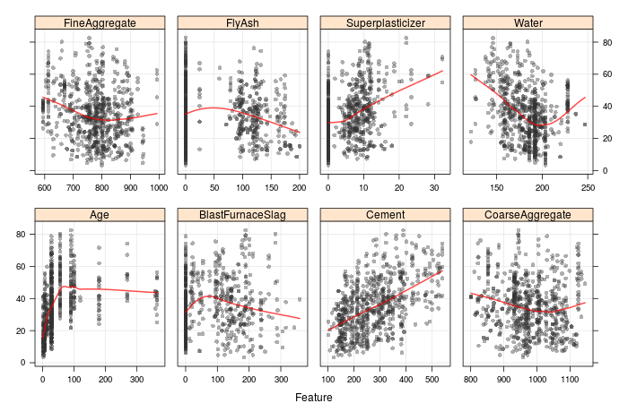
What can we see from these? A few interesting trends. Firstly, there are mostly non-linear relationships between the mixture ingredients and the compressive strength (cement is an exception here). We also see that there are many mixtures with zero superplasticiser, fly ash or blast furnace slag. Further, there are a few distinct values of age (known as a process factor, as it is not a mixture 'ingredient'), rather than a truely continuous distribution. Also, there are several values of water where many samples have that exact amount. These could represent important subgroups in the data, and we will revisit this when we continue the discussion to metafeatures and feature weighted stacking. It seems that Yeh compiled his data from numerous sources, where presumably different emphasis was placed upon the mixtures of interest.

Benchmark: averaged neural network

Well, now we have a good handle on our predictive inputs and how they relate to the outcome, lets consider how we will investigate building stacked regression models. I decided (probably because I have been using neural networks a lot recently) to fit multiple single-layered neural network models to generate the predictions to stack. In the APM book, the authors suggests that 27 units in the hidden layer is optimal, so I will take their word for it.

As a comment, Breiman suggests that stacking neural network models obtained from the same optimisation at diffent epochs in the optimisation process probably won't be effective. Here, my approach is different, as all the networks are seeded differently. As the cost function for a neural network isn't convex, they may converge with different parameters when fitting, so they will have a degree of independence from one another. These predictions are what Breiman refers to as 'level one' data. He produces his level one data in different ways; for example using leave-one-out cross validation combined with increasingly complex linear models, or with CART models.

I will comment that I had some issues with reproducibility; even explicitly setting the random seed seemed to yield different results. A little investigation suggests that it may be due to the parallel backend that I am using; the sub-processes can reset the seeds. Just a warning, if you run my script and get slightly different results.

So how well do neural networks perform? I built 20 models, each with one hidden layer and 27 units, explictly seeded differently from one another. We can train the models with this syntax:

#
# set cross validation method
#
ctrl <- trainControl(method = repeatedcv,
                    number = 10,
                    repeats = 5)
#
# define the training 'grid' 
# (only one set of parameters to be used)
#
nnetGrid <- expand.grid(decay = 0.001,
                        size = 27)
#
# train the models, and store in a list.
# seed is changed every time so different results
# will be obtained
#
models <- lapply(seq(1, 20), function(x) {
  set.seed(x)
  train(x = trainInput,
        y = trainOutcome,
        method = nnet,
        tuneGrid = nnetGrid,
        preProc = c(center, scale),
        linout = TRUE,
        trace = FALSE,
        maxit = 1000,
        trControl = ctrl)
})

and then plot the RMSE for the resamples (I used repeated ten-fold cross validation):

nnet-resamples

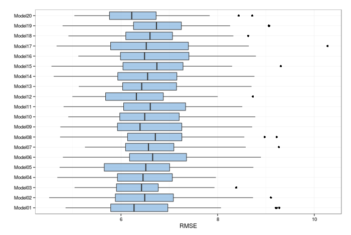
It seems that they are all centered around a RMSE of just over 6, with an interquartile range of about 0.5. A common trick with neural networks is to average them; that is, to combine the models with an equal weight. We get a RMSE of 4.549 on the validation set, and 3.828 on the test set (once again, the use of the parallel backend for training models hampers the exact reproducibility of these results). These can be seen as our 'benchmarks' to beat. I'll emphasise that I used simple averaging here, not bootstrap aggregation (or 'bagging'- another topic for another time).

As an aside, this is a prime example of why a single test set shouldn't be considered the 'best' test of the models performance; the results from the test and validation set are notably different from one another. Here, this is likely due to the limited sample size in each, but this result serves a word of warning none the less!

Basic Linear Stacking

Right, what is the idea for linear stacking? The first step is to fit the models on the training data. As we saw above, we have fitted 20 single-layer neural network models. Next, we want to make predictions on the validation set (note- I am calling this the validation set- its just my choice of naming convention). These predictions are our level one data. We then want to build a linear regression model with the level one data as the predictive inputs, and the true compressive strength as the outcome. Finally, we can make obtain our level one data (predictions) for the test set, and combine them using the coefficients we obtained when we performed the linear regression to stack the models.

The below plot shows the level one data (predicted validation set values) plotted against the validation set values. We do see some notable differences in the quality of performance, which definitely explains why averaging improves the quality of the regression, and hopefully it means that stacking will also be able to improve the predictive power of the model.

validation-predictions

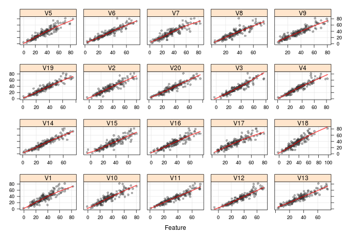
Breiman correctly points out there are some issues with this technique; notably, that the level one data will likey be significantly correlated, as here it is built from the same class of model trying to predict the same outcome. We will get round to addressing that shortly.

Following the procedure for basic linear stacking can be achieved using the syntax:

#
# set seed and train using caret::train
# valPred are the level one data (predictions on the 
# validation set), and valOutcome is the true 
# outcome of the validation set
#
set.seed(1234)
linearStack <- train(x = valPred,
                     y = valOutcome,
                     method = lm,
                     trControl = ctrl)
#
# combine results with test set outcome
#
lmStacked <- data.frame(predict = predict(linearStack, testPred),
                        actual = testOutcome)
#
# performance on test set:better than the indidividual models,
# not as good as averaging
#
caret::RMSE(lmStacked$predict, lmStacked$actual)
caret::R2(lmStacked$predict, lmStacked$actual)

I get a test set RMSE of 4.312, which is still a huge improvement on the level one data, but not as good as the benchmark equally weighted averaged results (a test set RMSE of 3.828 was obtained).

Linear Stacking with the Elastic Net

So, if our problem is with correlated predictive inputs, how should we deal with them? Easy: penalised methods. We could use the Ridge, Lasso, or both. I opted to use both; the so-called Elastic Net. The bonus of this method is that it can perform feature selection as well as penalisation, and in my experience generally performs better than the Ridge penalisation method.

We can train the model with the syntax:

#
# set the tuning grid (L1 and L2 penalties)
#
enetGrid <- expand.grid(lambda = seq(0, 0.1, 0.01),
                        fraction = seq(0.05, 1, length = 20))
#
# set the seed, and train
#
set.seed(1234)
enetStack <- train(x = valPred,
                   y = valOutcome,
                   method = enet,
                   tuneGrid = enetGrid,
                   trControl = ctrl)

The results improve significantly on the basic linear stacking: a test set RMSE of 3.713; a small, but notable improvement on the basic averaging approach (it may be significant in a Kaggle competition!).

I will mention once again that differences in seeding can effect this. On some occasions, I saw that the averaging approach outperformed the penalised stacked model; I think this is just an issue with validating models with a single test set, which is in this case, rather small. But at the very least, the stacked approach appears to be as good as averaging. What is apparant though, is using a penalised method to combine the models is more effective than a standard linear model.

Combination with non-negative weights

Now this is interesting. Breiman mentions that using penalised methods can be effective, but he advocates that combining models using non-negativity constraints is a good method to chose.

This will require a different approach- we will have to do some custom optimisation. Effectively, we want to average our models, but solve for the optimum choice of weights (i.e. a better vector of predictions would presumably carry a heavier weight then a very poor vector of predictions).

The base R optim() function comes to the rescue. We want to minimise over the weights α_k:

∑_n (y_n - ∑_k α_k z_kn)²

(apologies for the poor quality of equations in Markdown... I should probably look into a better alternative!). The weight α must always be greater than zero, and in my case I constrain it so the sum of the α_k must equal 1. I tackled the problem by firstly defining the function to minimise:

#
# This function returns the SSE of the ensemble based upon
# the weights for the predictions of each model.
#
# At the moment enforce sum to 1
# Note that we take as input weights for number of models -1
# as we can determine the last weight from all the others 
#
weightedStack <- function(modelWeights, trainPred, trainOutcome) {
  #
  # number of predictions (these are vectors)
  nPred <- length(modelWeights) + 1
  #
  # check proportions in correct range
  #
  for(i in 1:(nPred - 1)) {
    if(modelWeights[i] < 0 | modelWeights[i] > 1) return(10^38)
  }
  #
  # deduce the final weight
  modelWeights <- c(modelWeights, 1 - sum(modelWeights))
  #
  # this will be violated if the sum of the weights
  # doesnt add to one
  #
  if(modelWeights[nPred] < 0 ) return(10^38)
  #
  # we want this 'composite' SSE 
  #
  return(sum(trainOutcome - sum(modelWeights * trainPred))^2)
}

Then, we can make a wrapper function around optim() for the minimisation, using Nelder-Mead or simulated annealing, as we are dealing with a discontinuous cost function. The below function generates 50 starting configurations, and returns the weights that produce the minimum cost out of these 50. This function was modified from an example in the chapter in Applied Predictive Modeling; I won't take all the credit for the ingenuity!

#
# wrapper function around optim
#
optimWeights <- function(trainPred, trainOutcome) {
  #
  # how many models did we use to make predictions?
  #
  nPred <- ncol(trainPred)
  #
  # randomly build up vector of n weights
  # which add to 1. Build up nStart of these
  nStart <- 50
  weights <- vector('list', length = nStart)
  #
  # set up the initial weights (ensure they add to one)
  #
  for(i in 1:nStart) {
    draws <- as.list(-log(runif(nPred)))
    denom <- Reduce(sum, draws)
    weights[[i]] <- simplify2array(Map(function(x, y) x / y,
                                       draws,
                                       denom)
    )
  }
  #
  # collect the results
  #
  weights <- do.call(rbind.data.frame, weights)
  for (i in 1:ncol(weights)) names(weights)[i] <- i
  weights$SSE <- NA
  #
  # loop over starting values and optimise for
  # minimum SSE for each of these
  # Use SANN or Nelder-Mead as discontinuous function
  #
  for( i in 1:nStart) {
    optimWeights <- optim(weights[i, 1:nPred-1],
                          weightedStack,
                          method = Nelder-Mead,
                          control = list(maxit = 5000),
                          trainPred = trainPred,
                          trainOutcome = trainOutcome)
    #
    # select the best based upon min cost function
    #
    weights[i, 'SSE'] <- optimWeights$value
    weights[i, 1:(nPred - 1)] <- optimWeights$par
    weights[i, nPred] <- 1 - sum(weights[i, 1:nPred - 1])
  }
  #
  # output the set of weights that give the minimum SSE
  #
  weights <- weights[order(weights$SSE), ]
  as.vector(unlist(weights[1, 1:nPred]))
}

How does this method fare? On the test set, using these weights deduced from the validation set, I can make my predictions with:

#
# use vapply to quickly get predictions based on weights
#
weightedSum <- rowSums(vapply(seq(1:20),
                              function(x) {testPred[, x] * weights[x] },
                              numeric(148))
)

I get a RMSE on the test set of 4.063- better than linear stacking, and significantly better than the level one predictions. However, this isn't as good as stacking with the elastic net, or simple model averaging.

Feature Weighted Linear Stacking

This is the final topic I will investigate in this post! The concept of feature weighted linear stacking is discussed in detail here. My take on the approach is that you want to start by identifying 'metafeatures' that identify notable regions of data. For example, in the concrete data set many mixes have zero superplasticiser. So the meta feature I will adopt is a binary 0/1 for whether the mix has zero or non-zero superplasticiser.

As a comment, I investigated a few metafeatures, and this is the only one that gave consistent results that improved on stakcing with the elastic net. I think the metafeature generation and selection process is a bit of a black art, but hey, thats what makes data science and machine learning fun!

So with the vector of metafeatures (in this case there is only one), we add an extra one which is a constant 1- this will allow the origional level one predictions to be included. Next, we want to perform a grid expansion, where each level one preduction is multiplied by the metafeatures. As we have 2 metafeatures, and 20 level one predictions, we now have 40 inputs for our linear stacking. An elastic net model can then be trained to this data, as per the code below:

#
# define meta features
#
metas <- data.frame(meta0 = 1,
                    meta1 = ifelse(valInput$Superplasticizer == 0, 1, 0))
#
# function to create inputs (combining meta features with level one data)
#
fwInput <- function(metaFeatures, modelPredictions) {
  out <- matrix(NA,
                nrow = nrow(modelPredictions),
                ncol = (ncol(modelPredictions) * ncol(metas)))
  count <- 1
  for (i in 1:ncol(metas)) {
    for (j in 1:ncol(modelPredictions)) {
      out[, count] <- metas[, i] * modelPredictions[, j]
      count <- count + 1
    }
  }
  as.data.frame(out)
}
#
# obtain the feature weighted inputs
#
fwInputs <- fwInput(metas, valPred)
#
# use the elastic net to fit the feature weighted
# stacked model
#
set.seed(1234)
enetStackFW <- train(x = fwInputs,
                     y = valOutcome,
                     method = enet,
                     preProcess = c(center, scale),
                     tuneGrid = enetGrid,
                     trControl = ctrl)

So what is the final result? I get an RMSE of 3.710 on the test set- a further (if only marginal) improvement on the results when using the elastic net without metafeature weighting. But a marginal improvement can be what makes the difference, especially if you are battling for a million dollar prize!

We also have to consider the possibility that we are approaching the irreducible error for the system; it could be that due to uncertainties in measurements of compressive strength, that little further improvement is possible. We did investigate this when we saw variation in the measured compression strength for the same mixtures. Also, the problem of a single, fairly small test set is recurrant: how fair a test is this of the models performance? A larger training, validation and testing set would of course be preferred, but such is life that it is not always possible.

Other Thoughts

Overall, this has been a fun post to write- I enjoyed the little bit of research, and I hope that my interpretation of the techniques outlined in the two papers give some inspiration to anyone looking to try stacking regression models.

Here I only considered stacking neural network models; there is no reason why you couldn't combine various different types of model. That being said, stacking models with a low variance in their predictions may not be too helpful.

But anyway, I have found this to be a fun, educational experience, and I plan to investigate model ensembles in the context of classification models in the near future!

TL;DR- I investigated several ways to stack regression models, ranging from simple averaging to feature-weighted linear stacking.