27 Jan 2015

Churning with Caret: Trees and Rules

To briefly put this in context, I have been working through some exercises in Max Kuhn and Kjell Johnson's Applied Predictive Modelling book. In a previous posts, I looked at applying a set of linear models and non-linear models to a customer churn data set. The non-linear models proved to be far more suited to the challenge so far- lets see how well trees perform!

As per usual, I've put my script on my github for the interested reader. Let's get stuck in!

Overview

Trees are an odd class of model- unlike many that we have seen, they are not based around optimising a set of parameters for a predictive equation (or set of non-linear equations). They are implemented recursively, splitting the inputs into smaller and smaller groups based on various criteria, such as the Gini index or information theory. The purpose of this post isn't to explain how trees work, however- it's to demonstrate how to use them, so I will refer a good discussion to books like this and this.

Time for a strategy for our modelling. As I hope you have read my previous two posts on the subject, I am not going to bother drawing you the same pretty pictures again as I investigate the predictive inputs. Lets jump straight in, and discuss how the tree models implemented in R need to be fed their information.

The good news about trees and rule based models are that they are typically uber robust. If non-informative predictive inputs are thrown in, they simply won't make their way into the predictive equation. That doesn't mean we should be silly though. In our predictive factors, we know the costs are fully correlated with the minutes, so we should remove one of these (let's remove the costs as we did before). One reason for this is interpretability- if both are included, if a split is to be made in a decision tree, it will be random as to which is chosen if there are two fully correlated predictors. That muddies up any chance of interpretability.

Trees are also ace because they typically don't need data preprocessing, and can deal with all types of odd distributions in their predictive inputs.

They are also easy to interpret, as they kick out a series of if-then-else statements that follow the branches down to terminal nodes, which can be read off in a transparent way.

These sure sound like the best thing ever, right? Well, there is some bad- classical CART (classification and regression trees) in their purest form are rubbish. They produce unstable results (i.e. slightly different data might massively change the prediction equations they produce). Boo. But here is where some sneaky tricks come into play. Combined with ensemble methods, trees become some of the most powerful prediction models out there. I will be demonstrating the usage of random forests, bagged trees and boosted trees shortly.

The main drawback of these techniques as they are notorious 'black box' models, which are practically impossible to interpret. You fit them, then make predictions with them... but if you are after of a nice, interpretable prediction equation, you are out of luck. Another drawback is that they can take a long time to fit- which can be an issue if you have very large data sets.

Preprocessing and filtering

As I mentioned above, we can pretty much skip this step if we want. For trees, I would recommend filtering zero variance predictors, and predictors that are fully correlated with one another (for example, we will filter out the costs, as they are fully correlated with the minutes).

Just as a point, even though trees are very resistive to non-informative predictors, it doesn't mean they are invincible to them. A model built out of only informative predictors will probably always outperform one that includes some non-informative predictors. Also, imagine your predictive factors are expensive to collect. If you could demonstrate that you only need a fraction of them to build a reliable model, that could have implications for huge savings. We should always try and think about what is being put into a model (when possible- hard if you have thousands of predictive inputs!).

As I have eluded to several times before, I will write a blog post about more robust feature selection techniques in the near future!

Now, here is the interesting thing about most tree-based models. They can handle categorical predictive inputs differently to the linear and non-linear models we saw before. Before, we had to dummy up the categories, and its usual practice to remove one to prevent colinearity issues. The way many of the tree based models are implemented in R is that we can look at independent categories or grouped categories. For independent categories, we just dummy up as usual. For grouped categories, we leave the input as-is; the algorithm can split by multiple groups (i.e category one and two might be in the left branch, and three, four and five in the right).

The problem; there is not usually much guarentee that either strategy will be better than the other. So you may have to try both!

Models

We will consider four models: bagged trees, boosted trees, random forests, and C50. C50 can be implemented using rules or trees, so we will consider both in the tuning process.

The boosted trees are implemented with the gbm package, which performs stochastic gradient boosting. There are other boosting methods, such as adaboost and xgboost (very popular with the cool Kaggle kids at the moment)- I will probably write an entire blog post on these once I find the time to play around and compare the different methods.

For the models, we will have three sets of input data. The state category is the most concerning; looking at the log odds of churn for the different states, there could be some meaningful infomation:

#
# log odds for states
#
stateTab <- table(churnTrain$state, trainOutcome)
apply(stateTab, 1,
      function(x) log((x[1] / sum(x)) / (1 - (x[1] / sum(x)))))

However, there are so few customers from each state that I dont feel too comfortable including it in a model. As trees intrinsically perform feature selection, as a compromise, for independent categories (i.e. where we dummy up the categorical inputs) we will have one set that includes the state, and another that doesnt. For grouped categories (i.e. we leave categorical inputs as is) we have to remove the state, as some models (such as random forest) will accept a maximum of 32 levels for a catagorical input (for good reason, when you think about the number of possible splits).

As always, I really encourage looking at Max and Kjell's book for a decent description of how these models work, and then seek out the references within for more in-depth infomation.

As an example, the snippet below demonstrates how you might tune a C50 model with caret::train():

#
# C5.0 tuning grid 
# trials are number of boosting iterations
# model can be either tree based or rule based
# winnowing allows the model to remove unimportant predictors
#
c50Grid <- expand.grid(trials = c(1:9, (1:10)*10),
                       model = c(tree, rules),
                       winnow = c(TRUE, FALSE))
#
# here, we train using the data set split into
# independent categories
#
set.seed(476)
c50TuneI <- train(x = trainInputI,
                  y = trainOutcome,
                  method = C5.0,
                  tuneGrid = c50Grid,
                  verbose = FALSE,
                  metric = Sens,
                  trControl = ctrl)

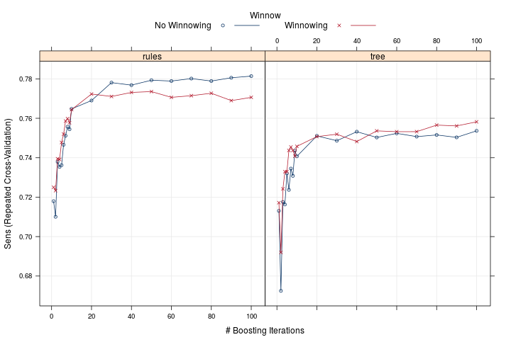
We see from plotting the resulting train object with plot(c50TuneI), that the rule based model with no winnowing performed the best. Little improvement was obtained beyond about 25 boosting iterations.

How did the models perform then? Below are the distributions for the resamples (I chose to do repeated 10-fold cross validation when training my models).

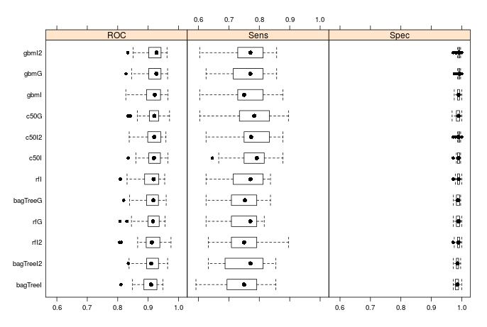
We see that typically, the version of the algorithm with independent groups without the states performs the best for each type of model. However, this isn't always the case- look at the random forest models. The usual saying is that 'there is no free lunch'- you can never guarentee a model's peformance on a specific data set. None the less, we see that all of the models have performed very well: the distribution of the area under the ROC curves are all centered above 0.9, the specificity is nearly 1 in all cases, and the distributions of the sensitivity (which we optimised in our training) are all centered between 0.75 and 0.8. Considering the ease of setup (we could have just blindly used the gbm model with grouped categories- that required barely any setup), this is pretty good. Remember how much preprocessing was needed for linear and non-linear models!

So how did the models perform on the test set? All of them actually did pretty well. The best was C50 with independent categories- it scored a sensitivity of 0.737, and the worst was C50 with grouped categories- it scored 0.683. All of the others were above 0.7. As always, I would present the argument that a single test set isn't neccessarily the best way to determine a model's peformance- best to take into consideration the peformance during resampling as well!

Variable Importance

We can look over the variable importance for the tree models using the usual syntax (see my previous two posts if usual doesn't mean anything to you!). The documentation for caret::varImp() specifies how these quantities are deduced.

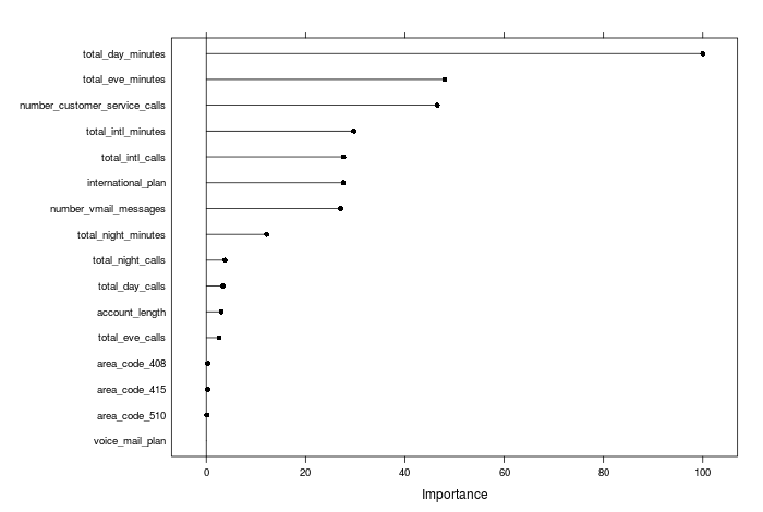
For the boosted tree (with independent categories, states not included) we see this ranking:

and for the random forest (with independent categories, states not included) we see this ranking:

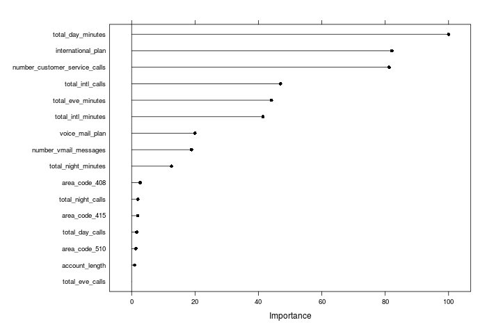
It is interesting to see that although they mostly rank the important predictors similarly, there are some marked differences; for example, the random forest model rates the number of international calls to be far more important than the boosted trees do. Overall, feature selection and variable importance can be very specific to the particular model you are using, and I will come back and investigate in a future post.

Model evaluation and comparisons

So what was the best model then? Overall, they all performed similarly during training and on the test set. Peforming t-tests between the resamples, we see that the boosted trees were better than the others, with p-values of less than 0.05. As the boosted trees performed nearly as well as c50 on the test set, I would select boosted trees with independent categories (without the customers' state) as my model of choice.

How do the calibrations look for our best models? The answer: not great.

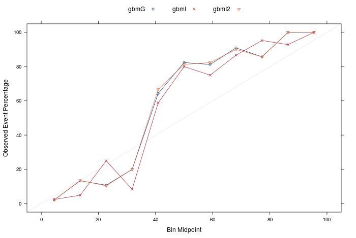
These calibrations are not good at all- and weren't really that great for any of the models. What does this mean? it means that we should be really careful interpreting the predicted probabilities as 'real' probabilities. This is where recalibrating the predicted probabilities would be useful - I will show how to do that in a future post.

That does not mean to say that our model is no good for predicting 'churn' or 'not churn'- it just means that if we were to go to our boss we would only really be able to say 'these will churn and these will not', instead of 'this group of customers will churn with 60% probability, this group with a 70% probability, etc'. The second scenario would be more useful; for example I might only be interested in targeting customers with a more than 70% chance of churning if budgets were tight and intervention expensive.

Finally, lets look at lift curves! Below is the plot for the best linear, non-linear and tree based model.

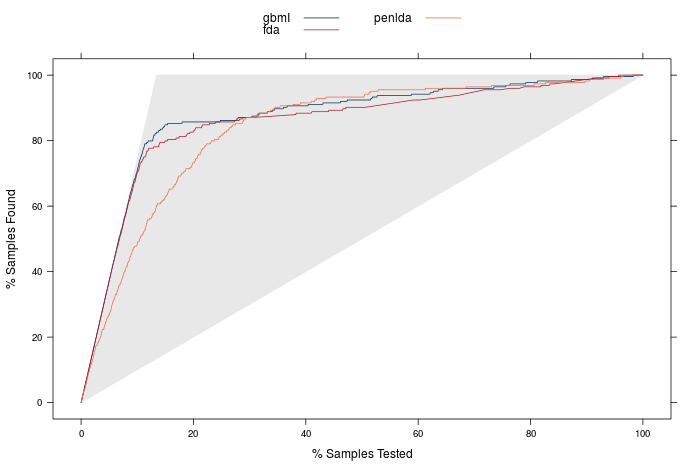
We see that our tree based model gives us that crucial extra bit of lift for finding the 80% of customers most likely to churn. We would have to contact about 12.5% (207) of customers to identify 80% of the total churners- so 179 of this 207 would actually churn. That gives us the edge over our best non-linear models!

Summary

Well, there we go. In a series of posts, we have looked at tree based models, non-linear models, and linear models to predict customer churn. We have looked at preprocessing, feature selection, and model evaluation. There have been several things that we may want to come back and visit, such as:

• supervised feature selection
• model calibration

Further, what about model ensembles? With our 'bag of models' that we could use, can we combine them so that they produce better results than our single best models? Looks like we aren't finished with you yet, churn data set!

TL;DR- I did some churn modelling, using tree and rule-based models. If you want my script of how I did it, it is here